Contents
- 1. Why test this on benefit formulas
- 2. What “weight-space programming” means here
- 3. Methods
- 4. Writing weights: exact, seven times
- 5. Replication: other writers, and the circuits underneath
- 6. Reading and editing weights
- 7. The control condition: trained networks fail structurally
- 8. The boundary: steps do not fit
- 9. Verification, and the corrections on the record
- 10. Limitations
- 11. What this means for evaluating AI in public benefits
- Reproducibility
- Footnotes
Weight-Space Programming for the Social Safety Net
An independent replication, with legal ground truth. The views represented here are my own. Last updated: November 2026
Executive summary
A November 2026 post by Tomita and co-authors, “Sparks of Weight-Space Programming,” reports that a frontier model can read and write the weights of a neural network directly, with no training.1 The claim is hard to evaluate on their examples because the tasks are benchmarks, where better is a matter of score. I tested the same three abilities (writing, reading, and editing weights) against US benefit formulas, where the correct answer is a matter of law and can be checked to the cent.
- Writing works. Seven benefit rules (SNAP, the earned income tax credit, SSI for individuals and couples, Medicaid patient liability and share of cost, and the Social Security benefit formula) were compiled into small network weights by construction. Every compiled network matched its statutory formula with a worst error under four trillionths of a dollar, across hundreds of thousands of test points.
- Other models can write them too. GPT-5.6 Sol and Gemini 3.1 Pro, given the rules as text, produced exact networks for nearly every rule. Given only the Social Security Administration’s published prose for a formula none of us had compiled before, all three writers returned the same eight parameters.
- Reading works, and editing is surgical. Models handed anonymized weights recovered the encoded constants exactly and flagged a planted defect (a stale prior-year parameter worth $51 a month). The defect lived in 2 of 1,297 parameters; editing those two restored exactness, producing a file identical to building the correct network from scratch.
- Trained networks fail differently. Networks trained on the same formulas posted small average errors and large structural ones. A trained SSI couple network changed a couple’s payment by up to $25.15 depending on which spouse earned the income, a distinction the law does not make, in 98.9% of equivalent households. Standard repairs shrank the defect without removing it. Building the rule into the architecture removed it. Compiling removed it and the error.
- There is a hard boundary. Benefit law contains steps (rounding rules, lookup tables, eligibility gates). A network computes a continuous function, and a continuous function cannot reproduce a step: for Social Security’s round-down-to-a-dime rule, no network can score better than $0.05 maximum error, and the best construction I built sits exactly at that floor.
Total API cost for the whole program: $2.48. Every experiment, including the failures and two corrected results, is public.2
1. Why test this on benefit formulas
The original post makes an extraordinary claim on the basis of an unreleased model, and its own results bound the claim in two places: editing weights did not give a model a capability it lacked, and one defect could not be identified from weights alone.1 A claim like that needs a test where the ground truth is not a matter of judgment.
Benefit formulas are that test. The SNAP allotment for a household is arithmetic specified in federal regulation, and the same is true for the earned income tax credit, Supplemental Security Income, Medicaid cost-sharing, and the Social Security benefit formula. If a model writes network weights that compute one of these rules, the weights are either right to the cent everywhere or they are wrong somewhere specific, and I can say where.
Small, specialized models are also my working territory. I trained a custom on-device redaction model that ships as a Mac app. I built a two-million-parameter speech-to-text model. So I ran this program the way I would want my own work run: protocols written before the experiments, pass/fail gates fixed in advance, failures published next to the successes, and every decisive number re-checked before this paper went out (Section 9).
These experiments cover the arithmetic cores of benefit programs. Who is eligible is a legal determination, and it belongs in deterministic, auditable code. The networks here are witnesses: independent implementations of a formula that can be compared against the production implementation, digit by digit. Nothing in this paper proposes that a neural network decide anyone’s benefits.
2. What “weight-space programming” means here
A small neural network is a list of numbers (weights) arranged in layers. Normally those numbers come from training: show the network many examples, measure its error, adjust. Weight-space programming skips training. Someone (or some model) works out what the numbers should be and writes them directly.
The networks in this paper are tiny multi-layer perceptrons with ReLU activations, which makes them piecewise-linear functions: assemblies of flat segments joined at hinges. Most benefit formulas are also piecewise linear. They are percentages of income segments, minus deductions, floored at zero and capped at maximums. That correspondence is the whole opportunity and, as Section 8 shows, also the boundary: a rule that is not continuous and piecewise linear does not fit.
Three abilities from the original post map onto three experiment families:
- Writing: produce weights that compute a stated rule, zero-shot, with no training.
- Reading: given weights with no labels, recover what rule and constants they encode.
- Editing: given weights containing a defect, change the defect and nothing else.
Each family gets a section below, followed by the control condition this kind of claim needs: networks trained the ordinary way on the same rules, tested for average accuracy and for the structural properties the law implies.
3. Methods
Pre-registration. Every experiment has a PROTOCOL.md written and committed before any weights were built or any API call was made. It fixes the rule as stipulated from primary sources,3456 the architecture, the scoring set, and the gate.
Gate. A construction passes if its maximum absolute error across the full scoring set is at most one cent. Partial credit runs to one dollar. Maximum error, not average error, is the primary metric throughout, because a benefit formula that is right on average and wrong for one household is wrong.
Scoring sets. Tens of thousands of points per rule: regular grids, uniform random draws, and dense sampling around every kink (the income values where a formula’s slope changes), since kinks are where approximations fail first.
Writers. The original constructions are mine, in the sense that this research program’s directing model (Muse Spark) derived them in-session and I reviewed and shipped them. The replication writers were OpenAI’s GPT-5.6 Sol and Google’s Gemini 3.1 Pro, called through OpenRouter under frozen prompts, one attempt each, with a single retry allowed only for unparseable replies.7 A refusal counts as a failure; one happened, and it is in the results.
Trained baselines. For each rule, a same-size network trained on examples from the true formula (Adam, cosine learning-rate decay, 15,000 steps of 8,192 samples), tuned honestly. The trained networks are the control that tells you what the ordinary method achieves on the same task.
Verification. Before this paper, I re-ran every experiment’s own scorer against the shipped weight files and compared the output with the published figures. Everything reproduced except one bound in one writeup, which is corrected and disclosed in Section 9.
4. Writing weights: exact, seven times
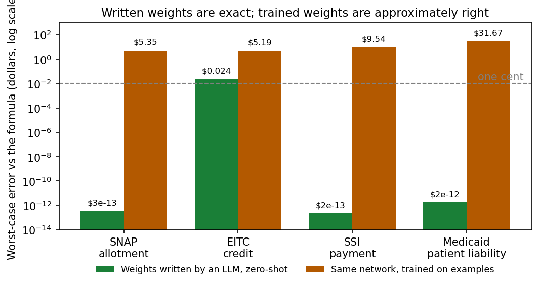
The first experiment took the FY2026 SNAP allotment for a household of two and compiled it directly: the standard deduction, the earned-income deduction, and the excess-shelter deduction became hinge units, and the 30-percent-of-net-income step became the output layer. No training data was generated and no gradient was computed. Scored on 40,049 points, the network’s largest error was 3.4e-13 dollars. That is floating-point noise, not approximation.
The same construction method then worked through the rest of the safety net:
| Rule | Test points | Max error (compiled) | Max error (trained) |
|---|---|---|---|
| SNAP allotment, household of 2 | 40,049 | 3.4e-13 | $5.35 |
| Earned income tax credit, 2 children | 2,818 | $0.024 (see below) | $5.19 |
| SSI payment, individual | 32,381 | 2.3e-13 | $9.54 |
| Medicaid patient liability | 86,105 | 1.8e-12 | $31.67 |
| Medicaid share of cost (California) | 43,607 | 1.4e-12 | $32.73 |
| SSI payment, couple | 44,762 | 5.8e-13 | $48.11 |
| SNAP with per-member inputs | 30,000 | 4.3e-13 | $64.60 |
Compiled vs. trained, maximum error by rule
Two of these results deserve a paragraph each.
The tax credit is a Partial, and the reason is informative. The compiled EITC network’s worst error is $0.024 at exactly one point, the top of the phase-out. The published rule says the credit reaches zero at $57,310 of income; the statute’s arithmetic actually reaches zero at $57,310.114, and the published figure is that value rounded to the nearest ten dollars. A network that implements the rounded endpoint inherits a 2.4-cent discontinuity. The construction was correct against the document it was handed; the document was rounded. This is the first appearance of a theme that dominates Section 8: published law contains rounding, and rounding is where exact representation goes to die.
The share-of-cost construction caught real errors elsewhere. California’s Medicaid share of cost reuses the SSI income-counting machinery, so the compiled network reused the SSI counting units verbatim and added one output stage. It reproduced, exactly, the two cases where my earlier audit work had found a benefits-as-code oracle returning wrong answers ($1,380 and $880 of share of cost, where the oracle had treated a positive share of cost as ineligibility). A compiled witness that agrees with the statute is most useful precisely when it disagrees with an existing implementation.
5. Replication: other writers, and the circuits underneath
A single model writing exact weights could be a party trick. The replication experiments gave the same rules, as text, to GPT-5.6 Sol and Gemini 3.1 Pro under frozen prompts.
Both models produced exact networks for SNAP, SSI (individual and couple), Medicaid liability, Medicaid share of cost, and the per-member SNAP variant, on first attempts. On the EITC, Gemini reproduced the original result exactly, including the $0.024 seam, which means it implemented the same rounded endpoint from the same text. GPT-5.6 Sol declined the EITC twice. It returned no weights, with a correct derivation of why the stipulated rule’s discontinuity made an exact continuous implementation impossible at that point. By the pre-registered gate that is a failure, and it is recorded as one. It is also the most interesting failure in the program: the model refused because it had found the seam.
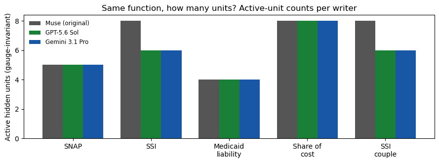
Agreement at the level of outputs could still hide different machinery. The canonical-circuits experiment asked whether the writers built the same network, by normalizing each construction under the two symmetries that relabel a network without changing its function (permuting hidden units, and rescaling a unit’s incoming and outgoing weights). Under that normalization:
- Medicaid liability and share of cost: all three writers collapse to one canonical circuit.
- SSI and the SSI couple rule: the two API writers share one circuit, leaner than the original construction.
- SNAP: the original and GPT-5.6 Sol share a circuit; Gemini’s computes the same function through genuinely different wiring.
Most cross-writer parameter difference is relabeling. Where it is not, the method says so: the EITC constructions, which implement slightly different functions because of the seam, correctly refuse to collapse.
Canonical circuits: which writers built the same network
6. Reading and editing weights
Reading. Eleven weight files were anonymized, hash-frozen, and handed to GPT-5.6 Sol and Gemini 3.1 Pro with no labels. Ten were compiled constructions from this program, including one with a planted defect. The eleventh was a trained network, included as a control.
On the compiled networks, both readers recovered the encoded rules and constants exactly, 100% of the constants, including thresholds stated to the cent. The planted defect was a network compiled with the 2024 SSI federal benefit rate ($943) in place of the 2026 rate ($994), the same class of stale-parameter error that audits keep finding in production benefit code. Both readers flagged it from the weights alone; one wrote that the network would “underpay by as much as $51 per month.”
The control is the honest limit. On the trained network, the readers named the right rule family but invented the constants ($1,000 and $914 for a ceiling that is neither). Reading works when the weights were written to be read. Trained weights smear their constants across every parameter, and no reader can recover what was never localized.
Blind weight reading: what the readers recovered
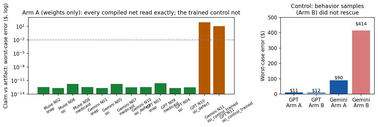
Editing. The stale-rate network differs from the correct 2026 network in exactly 2 of its 1,297 parameters, the two places the benefit rate appears as a literal. Changing those two numbers to the 2026 value restored exactness across the full scoring set, and the edited file is array-for-array identical to the independently constructed 2026 network. In the trained control, no parameter equals either rate; there is nothing to edit. A defect you can point to is a defect you can fix with a two-number patch and a regression test. A defect diffused through 1,297 numbers is a retraining run and a hope.
7. The control condition: trained networks fail structurally
Everything above could be read as a curiosity (of course a formula can be hand-coded into a network; hand-coding is what programmers do) until you run the control. The trained baselines are what machine learning actually produces when you point it at these rules, and their headline numbers look respectable. The trained SSI couple network has a mean absolute error of $0.32. Certified on average accuracy, it ships.
Then test the properties the law implies. SSI counts a couple’s combined income once: the $20 general exclusion applies to the couple, the payment cannot depend on which spouse earned what. Hold the couple’s total income fixed and vary only the split between spouses, across 121 splits in each of 90 income classes. The compiled networks, all three writers, do not move (worst variation 8.9e-13). The trained network moves in 98.9% of classes, by $3.64 on average and up to $25.15. Same household, same total income, payment determined by which name is on the paycheck. The worst class is diagnostic: at zero earned income and $250 of unearned income, the trained network’s answers fan out by the full $25.15, the fingerprint of a network that learned the $20 exclusion per person because most of its training couples had one earner.
Split invariance: same couple, same income, different split
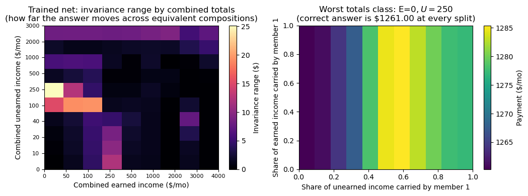
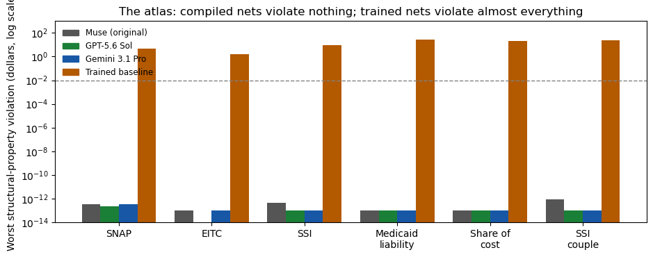
The structural-property atlas generalized this from one property to twenty-three property families (monotonicity in each input, output bounds, plateau flatness, exclusion ordering, split and swap invariance) across all six rules and all writers. No compiled network from any writer violated any property by more than 8.9e-13, and 0% of compiled probes were off by more than a cent. The trained networks violated properties everywhere: SNAP payments escaping their legal range on 21.5% of probes, the EITC plateau failing to be flat on 98.6%, the SSI first-$20 exclusion property failing on 100% of probes, Medicaid liability breaking monotonicity in every direction tested. They are the rule’s own logic, unlearned.
The structural-property atlas
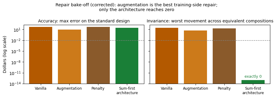
Can training be repaired? The bake-off took the couple defect and tried the standard fixes. Training on split-augmented data (the same totals at many splits) cut the worst split-dependence from $25.15 to $5.30 and produced the most accurate learned network (max error $8.98), but 95.6% of classes still moved. An explicit symmetry penalty in the loss did worse than augmentation on nearly every measure (max error $48.07, split-dependence $19.28); my pre-registered expectation that the penalty would win was wrong, and the writeup records it as wrong. An architecture that sums the two incomes before anything else sees them achieved split-invariance exactly, zero movement in every class, because the defect became unrepresentable, though its ordinary accuracy stayed mediocre (max error $25.14). Only compilation removed the defect and the error together.
The repair bake-off
Average error is a measure of how a model does on the distribution you tested. Property violations are measures of whether it learned the rule at all. An evaluation that reports only the first will certify systems that treat identical households differently, and it will do so with a clean conscience and a good score.
8. The boundary: steps do not fit
Every rule above is continuous. Benefit law is not. It rounds, it looks values up in tables, and it gates eligibility categorically. The final pair of experiments maps that edge, using the Social Security benefit formula because the SSA’s own text contains both halves of the story.
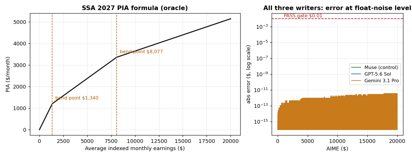
The held-out half. For the first seven rules, I restated each formula in clean form before any writer saw it, which left the strongest objection open: the writers were handed the answer as an equation. So the last writing test used a rule nobody in this program had compiled (the Social Security primary insurance amount for workers first eligible in 2027, in the form SSA currently publishes) and handed the writers only the SSA’s published prose: percentages and bend points in words, retrieved verbatim from ssa.gov.6 GPT-5.6 Sol, Gemini 3.1 Pro, and the control construction all returned exact networks on first attempts, worst error 3.6e-12 across 120,003 points. All three returned the same eight nonzero parameters. Prose in, identical circuit out, three for three.
Held-out test: the 2027 Social Security formula from prose
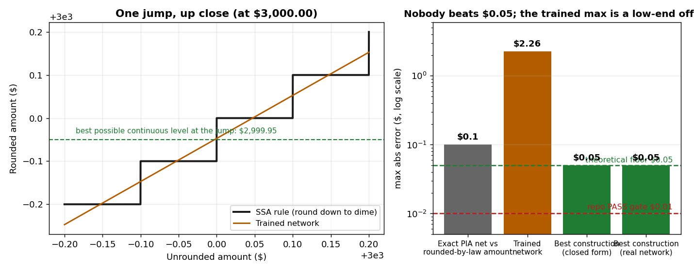
The rounding half. The SSA text ends with an instruction I had told the writers to skip: “We round this amount to the next lower multiple of $.10.” That rounding is a step function, and a ReLU network computes a continuous one. The incompatibility is exact. At a jump of size J, a continuous candidate takes a single value at the jump point, while the truth differs by J across it, so the candidate’s maximum error is at least J/2 no matter how it is built or trained. For the dime rule the floor is $0.05. For the whole-dollar rounding of the monthly benefit, it is $0.50. For a categorical eligibility gate, where the jump is the entire decision, approximation language stops being meaningful.
Measured against that floor: the best construction (flat everywhere, ramping through each jump’s midpoint in a hairline interval) attains exactly $0.0500 maximum error and is within a cent 99.2% of the time. It is optimal, and it still cannot pass a one-cent gate, ever. The trained network independently found the midpoint strategy (mean error $0.0250 across the middle of the range) and added a defect of its own at the bottom of the range, an offset worth $2.17 at zero that training shrank but did not remove. And the exact PIA network from the held-out test, scored against what the law actually pays after rounding, is off by up to $0.0999 with a mean of $0.051: the rounding gap itself, incurred by a pipeline that is exact at every step a network can represent.
The rounding boundary
The boundary statement for the whole program is now precise. Continuous, piecewise-linear rules (the arithmetic of benefit formulas) are exactly representable as weights, and current frontier models can write, read, and edit those weights reliably. Discontinuous rules (rounding, tables, gates) are representable only to half their jump size. A sound system uses each where it belongs: deterministic code for determinations and rounding, compiled weights as cross-checks on the arithmetic, trained models nowhere near either unless their property tests pass.
9. Verification, and the corrections on the record
A result you cannot re-derive is a claim. Before this paper was drafted, every experiment’s scorer was re-run against the shipped weight files and compared with the published numbers (full table in the repository’s VERIFICATION.md). The exact constructions, the $51 defect and its edit, the $25.15 split-dependence, the bake-off, the circuit equivalences, and the held-out result all reproduced to the digits originally reported. The weight-reading artifacts match their frozen hashes, 11 of 11.
Two corrections stand in the record, and they belong in the paper rather than under it.
First, the bake-off’s original internal report contained two figures from a corrupted result delivery (a symmetry-penalty result of $11.28 that was never real, and a sum-first result described as the most accurate arm, which it is not). The shipped weight files were re-scored in the foreground, the results rewritten with an erratum, and the corrected figures (penalty $19.28 split-dependence; augmentation, not sum-first, is the best learned arm) are the ones in Section 7. The lesson is now a standing rule for this work: a background success report is not evidence, and decisive numbers get re-produced against the artifacts before they are published.
Second, the verification rerun itself caught the atlas writeup overstating a bound: compiled property violations were described as “at most 4.4e-13,” and the SSI couple original’s worst probe is 8.9e-13. The sentence is corrected in place. Nothing depends on the difference; both numbers are a trillionth of a dollar. It is disclosed here because a paper about checking numbers should survive its own standard.
10. Limitations
- The networks are tiny and the rules are the easy class. Everything exact in this paper is a small piecewise-linear function. Real benefit systems compose dozens of such rules with categorical gates, household data, and state variations. The witness method scales by composition (the share-of-cost network reused the SSI counting machine verbatim), but nobody should mistake seven arithmetic cores for a benefits system.
- The headline model from the original post is untested. GPT-6 Astra is unreleased. The writers here were GPT-5.6 Sol, Gemini 3.1 Pro, and Muse Spark. This paper replicates the write/read/edit claims with available models; it says nothing about the original team’s system.
- The capability-improvement claim is untested. The original post’s most ambitious result, improving a model’s benchmark performance by editing weights, is untouched here, and their own report shows it failing where the capability was absent. Nothing in this paper bears on it.
- The writers may know these formulas. SNAP and SSI arithmetic is public and heavily documented; the held-out test used the 2027 Social Security formula in its currently published form, and a writer that has memorized it still has to produce exact weights, which is the ability under test. But this program measures weight-writing, not rule discovery from ignorance.
- One refusal is one data point. GPT-5.6 Sol’s EITC refusal was scored as a failure by the gate and reads as discernment in the prose. Both readings are recorded; neither should be generalized from a single instance.
11. What this means for evaluating AI in public benefits
Three conclusions survive every caveat above.
Test properties alongside accuracy. The trained couple network’s $0.32 average error and its $25.15 split-dependence are both true statements about the same artifact. An evaluation program that measures the first and not the second will certify a system that treats identical households differently, and the failure will surface as an appeal, a fair-hearing loss, or a headline, in ascending order of cost. The properties are not hard to enumerate: whatever the law says cannot matter (which spouse earned it, the order members are listed in, the order facts are presented in) must not move the answer. Write those tests before the accuracy tests.
Independent witnesses are a cheap audit. A compiled witness costs cents to produce, runs in microseconds, and disagrees with a production system at exactly the inputs where one of them is wrong. It caught a real oracle’s errors in this program (Section 4) and its own author’s rounded endpoint (the EITC seam). Agencies already cross-check benefit calculations by hand on a sample basis; a witness does it exhaustively, on every release, for the price of a coffee per rule.
Keep the boundary in the architecture. Determinations, gates, and rounding belong in deterministic code, not because models are untrustworthy in some general sense, but because Section 8 is a proof: a continuous system cannot represent them, full stop. The design question for AI in benefits is which side of that line each component sits on, and whether the evaluation can tell the difference.
Determinations stay in deterministic code, and the burden of this paper is that we can now say, to the cent and in one case to the trillionth, exactly why.
Reproducibility
All protocols, weight files, scoring code, raw model replies, and cost logs are in the public repository.2 Every experiment’s RESULTS.md carries its own cost line; the program total is $2.48 of API spend, with the remainder run locally. The figures in this paper are the experiments’ own. Nothing was retrained or re-scored for this writeup beyond the verification pass described in Section 9.
Footnotes
-
Tomita, R., et al. “Sparks of Weight-Space Programming.” November 2, 2026. https://rikiyat.github.io/blog/weight-space-programming/ ↩ ↩2
-
Trimm, C. “Weight-Space Programming for the Social Safety Net” (code, weights, protocols, and data). GitHub, 2026. https://github.com/ctrimm/weight-space-programming ↩ ↩2
-
SNAP FY2026 parameters: maximum allotments, standard deduction ($209 for household sizes 1–3), and the excess shelter deduction cap ($744), per USDA FNS cost-of-living adjustment guidance for fiscal year 2026. ↩
-
Earned income tax credit, tax year 2025, two qualifying children: 40% phase-in to $17,880, maximum credit $7,152, phase-out at 21.06% from $23,350 to the completed phase-out amount of $57,310, per IRS parameters for tax year 2025. ↩
-
SSI 2026: federal benefit rate $994 (individual) and $1,491 (couple), with the $20 general exclusion and $65-plus-one-half earned income exclusion, per SSA. Medicaid patient liability per 42 CFR 435.725, with the 2026 minimum monthly maintenance needs allowance of $2,643.75 and a stipulated $50 personal needs allowance. California share of cost per the state’s Medi-Cal rules (maintenance need $600 for a single person, SSI counting methodology). ↩
-
Social Security primary insurance amount, workers first eligible in 2027: 90% of the first $1,340 of average indexed monthly earnings, 32% of earnings over $1,340 through $8,077, and 15% above $8,077, rounded down to the next lower multiple of $0.10. Social Security Administration, “Primary Insurance Amount,” retrieved November 3, 2026. https://www.ssa.gov/oact/cola/piaformula.html ↩ ↩2
-
Model identifiers as served by OpenRouter:
openai/gpt-5.6-solandgoogle/gemini-3.1-pro-preview. Prompts, raw replies, and per-call costs are preserved in each experiment’s folder in the repository. ↩
Related Posts
- Reviewing the 2024 Federal AI Use Cases InventoryDiving into the massive 2024 Federal AI Use Cases Inventory to see how government agencies are actually using AI. Over 2,100 use cases? Let's break it down.3/9/2025
- Little AI Projects: Experiments at the Intersection of Government, Civic Tech, and ProductivityA roundup of small AI experiments I've been building - MCP servers, benefits navigators, policy engines, and local model fine-tuning - all exploring how AI can make government more accessible.3/12/2026
- Using Synthetic Government Benefits Data for Reasoning EvaluationWhy the question isn't 'can the model do arithmetic?' but 'does it know which rule to apply?'. Exploring synthetic data for evaluating reasoning in government benefits policy.3/27/2026